this link. Thank you! 😸

Links to our paper:

• TMLR: https://openreview.net/pdf?id=qqnttX9LPo
• ArXiv: https://arxiv.org/abs/2307.01452

Tutorial:

• Causal Reinforcement Learning: Empowering Agents with Causality

Github Project (We will keep this project regularly updated.): Feel free to give us a star ⭐ if you found this helpful. We also greatly appreciate everyone contributing together! 😊

• Awesome-Causal-RL: A curated list of causal reinforcement learning resources.

Preface

This time, I’d like to share with you the recent publication of our comprehensive review paper on Causal Reinforcement Learning (Causal RL), which has officially been accepted by Transactions on Machine Learning Research (TMLR). Causal RL is an intriguing, burgeoning field that centers on empowering agents to better comprehend the causality within an environment, thereby enabling them to make more informed and effective decisions. In this blog post, alongside delving into segments of our survey paper, I’ll also briefly share some reflections on this topic. To keep our discussion focused, let’s establish a few key points:

1️⃣ A Fact: Agents Still Lack Understanding of Causality

By the end of 2023, agents still struggle considerably in grasping causality. ChatGPT stands as one of the most advanced agents based on LLMs. Let’s use it as an example:

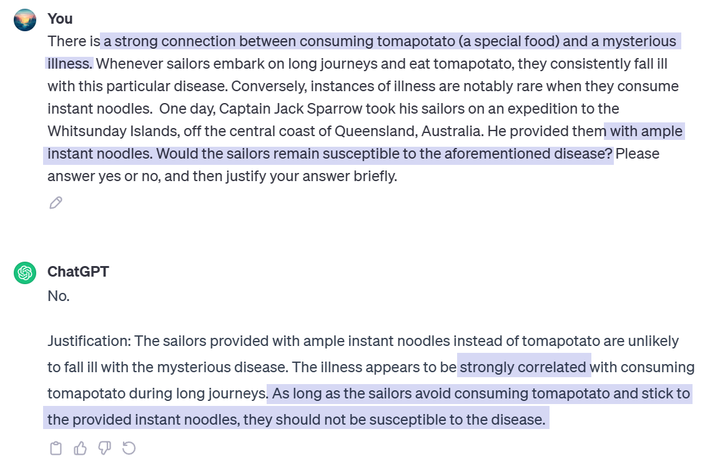
A failure case of ChatGPT.

In this example, we created a hypothetical food called ‘tomapotato’ and shared with ChatGPT a supposed connection between eating this food and developing a mysterious disease (correlation). Additionally, we pointed out that individuals who regularly eat instant noodles rarely suffer from this disease. We then asked ChatGPT about whether sailors would fall ill with this disease if they had plenty of instant noodles (causality). ChatGPT ‘smoothly’ fell into our prepared trap and responded: ‘As long as the sailors avoid consuming tomapotato and stick to the provided instant noodles, they should not be susceptible to the disease.’ This is a classic case of mistaking correlation for causation. It’s noteworthy that if we were to replace this scenario with a historically accurate example—replacing tomapotato with contaminated meat and the mysterious disease with scurvy—ChatGPT would provide the correct answer. This example has been documented in various sources, so ChatGPT’s correct response isn’t surprising. However, minor alterations could mislead such a state-of-the-art agent, rendering its responses unreliable and potentially causing real risks. This emphasizes the need for reflection and further investigation.

Similarly, researchers from TU Darmstadt mentioned a phenomenon in their paper recently published on TMLR¹:

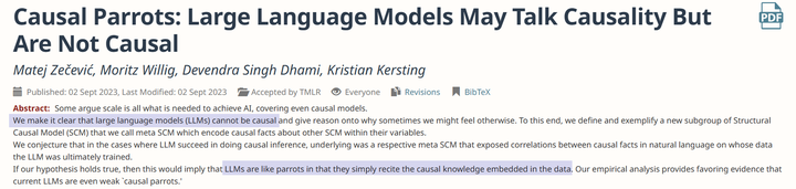
LLMs are `causal parrots.`

The authors referred to this phenomenon as ‘Causal Parrots.’ In simple terms, this implies that even the most powerful agents, although they might exhibit human-like behavior, are merely repeating causal knowledge that already exists in the training data, without genuinely understanding it, much like parrots mimicking speech.

2️⃣ A Value: Agents Should Understand Causality

While acknowledging the aforementioned facts, we sometimes hear a voice suggesting that intelligent agents do not need to understand causality since humans make mistakes about causality as well. Sometimes, decisions based on correlation alone seem satisfactory, so why bother pursuing causality for agents? Although agents like ChatGPT don’t fully grasp causality, it doesn’t stop them from quickly becoming an indispensable part of many people’s workflow. In the task of conversation, leveraging internet-scale data, sufficiently large model capacities, and proper alignment, many tasks based on natural language seem to have been solved. However, we believe there remains a significant gap between ‘usable’ and ‘reliably usable.’ If we hope for intelligent agents to more deeply engage in human society, particularly in making important decisions related to humans, we cannot settle for ‘usable’ but must forge a new path toward ‘reliably usable’—and Causal RL may be such a path. To quote Judea Pearl²:

I believe that causal reasoning is essential for machines to communicate with us in our own language about policies, experiments, explanations, theories, regret, responsibility, free will, and obligations—and, eventually, to make their own moral decisions.

Therefore, it is valuable for agents to understand causality, and it’s definitely something worth pursuing. The value is not only reflected in enabling agents to naturally communicate their choices and intentions with humans but also in enhancing our trust in agents, freeing us from the fear of super artificial intelligence.

3️⃣ A Method: How to Enable Agents to Understand Causality? Still Under Research

While we may reach consensus on the previous two points, the third one admits various answers. Should we impart causal knowledge to artificial agents directly, or merely offer serveral first principles for them to learn on their own? Should agents learn causality through interacting with the environment or by studying historical data alone? Should causal reasoning modules be integrated internally within the agent, or should they exist as external tools? Each distinct choice can lead to many intriguing solutions, employing differing techniques. In the survey, we organized the existing work on causal RL based on four major problems: enhancing sample efficiency, advancing generalizability and knowledge transfer, addressing spurious correlations, and promoting explainability, fairness, and safety. As research on agents continues to evolve, new challenges will emerge, and we genuinely welcome everyone to contribute and share your thoughts and insights on this topic.

Before diving into the main content, let’s add a bit of fundamental knowledge to help understand how causality is formalized mathematically.

Background Knowledge

First, let’s introduce Judea Pearl’s Structural Causal Model (SCM)³:

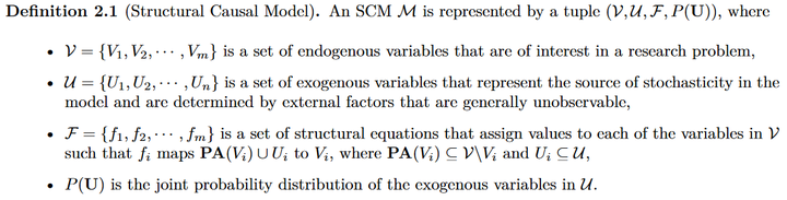
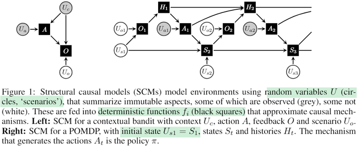
This is a tuple comprising an endogenous variable set, an exogenous variable set, a set of structural equations, and the joint distribution of exogenous variables. Endogenous variables are the ones we are interested in a research problem, such as the states and rewards in an MDP (Markov Decision Process). Exogenous variables represent the ones we don’t specifically care about, also known as background variables or noise variables. These variables are linked through structural equations. Each structural equation specifies how an endogenous variable is determined, where the variable on the left side of the equation is the effect, and the endogenous variable on the right side represents the corresponding causes. Because the equations themselves are deterministic, all randomness stems from exogenous variables. As a result, given the values of all exogenous variables, the values of endogenous variables are determined. In this way, an SCM describes the regularities of how a system (or the world) operates, enabling us to leverage it for discussing and understanding various causal concepts.

Earlier, we mentioned that ‘correlation does not imply causation,’ and we can better grasp this distinction using a pie chart:

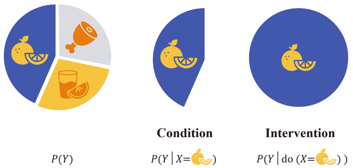
Suppose the complete pie chart corresponds to the population we are interested in, such as all sailors. This population can be divided into three sections based on the consumption of different foods, which we denote as variable $x$, and then use variable $Y$ to indicate whether they get the disease. The question we want to ask is: does consuming a certain food make sailors more or less likely to get the disease? In traditional machine learning, we might attempt to establish a predictive model to fit the conditional distribution $P(Y \vert X)$. However, the conditional distribution only studies a single section; it can answer questions about correlation, for instance: if we (passively) observe sailors consuming a certain food, how likely are they to get the disease? Yet, what we are actually interested in is a causal one: what changes if we (actively) conduct a certain intervention? To distinguish between the two, researchers introduced the do-operator. The intervention distribution $P(Y \vert \text{do}(X=x))$ represents how likely all sailors are to get the disease when they are required to consume a certain food. It might seem like a slight difference, but it’s crucial. If a model can only answer questions about correlation, it will be challenging to derive reliable conclusions from its predictions. This correlation could potentially arise from some confounding factor omitted by the model (e.g., a common cause of A and B). Perhaps consuming the food itself doesn’t lead to the disease, but an unknown gene makes people both prefer this food and be more susceptible to the disease (which would create a spurious correlation between the two). If all sailors consume this food without being influenced by some unknown cause, we can figure out this mystery. In the language of SCM, $\text{do}(X=x)$ removes the structural equation of $X$ and directly sets its value as $x$, thereby creating a world that meets $X=x$ with the smallest difference from the original world.

Perhaps someone might ask: Is it really feasible to force all sailors to consume the same food? This approach seems unrealistic and unethical. If we cannot achieve this, how can we ensure that the model learns the intervention distribution we are truly interested in? This brings up one of the most important achievements in causal science — how to predict the effects of an intervention without actually enacting it. To explain with the previous example, we can express assumptions in the form of a causal graph, where each node represents an endogenous variable, and the presence or absence of edges represents our assumptions about causal relationships. $X \rightarrow Y$ represents our assumption that consuming a certain food might lead to a disease. $X \leftarrow Z \rightarrow Y$ represents our assumption that there exists a confounding variable $Z$, which affects both the food consumed and the likelihood of getting the disease. In this way, we can obtain Figure 3.3:

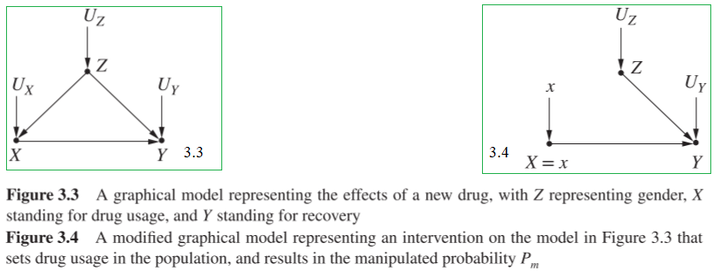
Similarly, to express that all sailors are forced to consume the same food, we can remove the edge $X \leftarrow Z$ from Figure 3.3 to obtain Figure 3.4. In other words, Figure 3.4 represents an intervened world, where the intervention distribution $P(Y \vert \text{do}(X=x))$ we care about is equivalent to the conditional distribution $P _m(Y \vert X=x)$. Leveraging basic knowledge of probability theory, we can make the following deductions:

The third equality relies on the assumption that $X \rightarrow Z$ doesn’t exist, meaning that changes in variable $X$ don’t lead to changes in variable $Z$, so the conditional probability equals the marginal probability. The fourth equality is based on two invariances: the marginal probability $P(Z=z)$ remains unchanged before and after intervention since removing $X \leftarrow Z$ doesn’t affect the value of $Z$; the conditional probability $P(Y=y \vert X=x, Z=z)$ remains unchanged before and after intervention because whether $X$ changes spontaneously or is fixed to a certain value, the structural equation for $Y$ (the process that generates $Y$) remains unchanged. So, what’s the use of this conclusion? It precisely solves the problem that had been bothering us earlier. Looking at the right side of the equation, we can see that both terms are common probabilities, without any do-operator or subscript ‘$m$’. This means we can use observational data to answer causal questions! Of course, in reality, variable $Z$ may not always be observable, so sometimes the causal effect of interest is unidentifiable.

Apart from intervention, there’s another highly important concept in causal science: counterfactual. In traditional machine learning, we seldom discuss this concept, but it’s quite common in our daily lives. Continuing from the previous example, after observing sailors who consumed “tomapotato” falling ill with a mysterious disease, we often contemplate a question: What would have been the outcome if these sailors hadn’t consumed “tomapotato” initially? Traditional statistics lacks a language to articulate such a question because we can’t precisely characterize “traveling back in time” (if … initially) and “intervention” (hadn’t consumed) solely through passively observed empirical data. To articulate the correct question, we must consider causal relationships and go one step beyond intervention. Why is that? With the aid of the do-calculus, we can attempt to write down the question as:

We can see that there are two $Y$s in this expression, each with different meanings. The first $Y$ represents the outcome when sailors do not consume ‘tomapatato,’ while the second $Y$ means the actual outcome of sailors consumed ‘tomapatato.’ To differentiate between these two scenarios, we need to introduce a new language called ‘potential outcomes.’⁴ This involves using subscripts to specify the values of specific variables. For an individual $u$, we can denote their potential outcome if they consumed ‘tomapatato’ as $Y _{X=x}(u)$ and their potential outcome if they did not consume it as $Y _{X=x’}(u)$. Obviously, for the same individual, we can only observe one potential outcome (the outcome in the factual world). For those unobserved potential outcomes, we can imagine they are the ones observed in parallel worlds (counterfactual worlds). Through potential outcomes, we can express the quantities of interest as follows:

Here, we first combine the condition $\text{do}(X=x’)$ into the target variable $Y$ to obtain $Y _{X=x’}$, as this is the actual variable of interest. Then, we completed the conditions; the original condition $Y=1$ refers to $X=x$ and $Y _{X=x}=1$. Moreover, since the potential outcome expressed by $Y _{X=x}=1$ aligns with the condition $X=x$, we can rewrite this probability as:

This expression represents: “If we observe $X=x, Y=1$, what would be the outcome in the world of $X=x’$?” This is precisely the question we want to ask. Using SCM, we can calculate this counterfactual quantity through three steps: first, we infer the values of exogenous variables $U$ based on known facts $X=x$ and $Y=1$; then, we modify the structural equations according to $\text{do}(X=x’)$ to establish a parallel world; finally, by substituting the values of $U$ into the modified structural equations, we can calculate the value of the counterfactual variable. This process itself is transparent, so counterfactuals are not just a hypothetical concept; they can be rigorously characterized using mathematical language. However, because SCM is typically unknown in practical applications, this process might not always be applicable. In such cases, we often rely on qualitative assumptions (such as causal graphs) to assist in computations involving counterfactuals.

So far, we’ve introduced SCM, which provides a way to mathematically model a world following specific causal mechanisms. We emphasized the distinction between correlation and causation, introducing interventions and counterfactuals based on SCM. These concepts aren’t merely jargon; they address the limitation in traditional statistics which focuses on correlation rather than causation. Will a new recommendation algorithm increase click-through rates and user retention? Would a patient have recovered better if they hadn’t undergone a specific treatment? Does a university’s admission decision involve gender or racial bias? These are all causal questions and they drive scientific and social progress. Consider a world governed by correlation rather than causation, where we might be attacked by sharks because we eat more ice cream or avoid seeking medical treatment due to a fear of death. Such a world would be absurd.

Okay, the basics end here. Causal science is an extensive field with many concepts, terminologies, and techniques worth exploring. However, to keep this post concise, we won’t delve further into it. 🕊️ Interested readers can refer to related books³⁵, our survey paper and blogs for more information:

Zhihong Deng：【干货】《统计因果推理入门》读书笔记

Back to the topic of reinforcement learning, after going through the content on causality, you might have some thoughts:

1. What is the connection between policy in reinforcement learning and intervention in causality?
2. What about the environmental model in model-based reinforcement learning (MBRL) and the causal model we mentioned earlier?

Being able to instantly come up with these two questions demonstrates your sharp thinking! 😎💡Firstly, in reinforcement learning, the process of interaction between agents and the environment is itself a form of intervention. However, this intervention typically doesn’t directly set the action variable $A _t$ to a fixed value but retains its dependence on the state variable $S _t$. Since we acknowledge that a policy respresents a form of interventions, a natural question arises: Does reinforcement learning itself learn causal relationships? For on-policy RL, agents indeed learn the total effect of actions on outcomes, and the fact that on-policy methods generally perform better than off-policy methods supports this point. However, it’s essential to recognize that the environment itself contains other types of causal relationships, such as the causal relationships among various state dimensions in adjacent time steps. Without understanding these causal relationships, the ability of agents will be limited to a single fixed environment. When the environment changes (e.g., due to external interventions affecting other factors in the environment), its performance decreses significantly. Regarding the second question, although traditional MBRL learns the environment model (sometimes referred to as the world model), it stops at the level of correlations. Once unobservable confounding factors show up, the learned model would become unreliable (think about the earlier example).

At the end of this section, we present the definition of causal RL used in the paper:

Definition (Causal reinforcement learning). Causal RL is an umbrella term for RL approaches that incorporate additional assumptions or prior knowledge to analyze and understand the causal mechanisms underlying actions and their consequences, enabling agents to make more informed and effective decisions.

The definition is broad, focusing primarily on two aspects: first, it emphasizes an understanding of causal relationships rather than superficial correlations to enhance agents’ decision-making abilities; and second, to achieve the former, causal RL usually requires incorporating additional assumptions and prior knowledge. Unlike other domains such as meta RL or offline RL, causal RL does not have a unified problem formulation or strive to solve a certain type of task. The research in causal RL typically flexibly designs solutions tailored to certain difficulties in a research problem. Therefore, in our survey, we adopt a problem-oriented taxonomy to organize the existing work on causal RL: 1) sample efficiency; 2) generalization and knowledge transfer; 3) spurious correlations; 4) exaplanability, fairness, and safety. Next, I will select a few papers to briefly illustrate the new perspectives that causal RL offers on these issues.

Sample Efficiency

First, we know that sample inefficiency is often criticized in reinforcement learning. There has been a considerable amount of research centered around improving sample efficiency, and here, I’ll introduce two works related to causal RL.

The first one was presented at NeurIPS 2021, titled “Causal Influence Detection for Improving Efficiency in Reinforcement Learning.”⁶ It deals with a robotic manipulation problem:

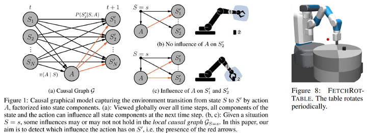
In reinforcement learning, the state space is usually considered as a whole. However, it can be decomposed based on the physical meaning of state dimensions, where each part corresponds to an entity, such as the end effector of a robotic arm or objects on a table. For robotic manipulation tasks, an agent must establish physical contact with an object to succeed. Only then can it potentially move the object to a target location. From a causal perspective, the essence of establishing physical contact is whether actions can causally influence objects. Therefore, we can construct a causal quantity to assess the effect of actions on objects, referred to as ‘causal influence’ in the paper. Based on causal influence, we can guide the agent on how to explore the environment more effectively —— prioritizing exploration in areas where physical contact with objects can be established, thereby improving sample efficiency. This approach is straightforward and effectively prevents the agent from engaging in meaningless exploration in the vast state-action space (e.g., randomly waving its arm in the air).

The second work I want to discuss here is DeepMind’s paper accepted by ICLR 2019, titled “Woulda, Coulda, Shoulda: Counterfactually-Guided Policy Search.”⁷ It studies an episodic POMDP problem:

The idea is quite simple: Many existing MBRL methods synthesize data from scratch. However, a common human practice involves leveraging counterfactual reasoning to make full use of experiential data. For instance, after encountering a failure, we often contemplate changing a previous decision at some point in time to alter the outcome. This mode of thinking significantly improves our learning efficiency. Similarly, we aim for agents to harness the power of counterfactual reasoning as well:

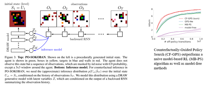
The experimental environment is Sokoban where the green entity represents the agent. A visible area of 3×3 cells centered around the agent is observable, while the rest of the map is masked with a 90% probability, making it a POMDP problem. The authors employed an idealized setup assuming known dynamics, allowing the agent to focus on reasoning the distribution of exogenous variables. The experimental results effectively validated the effectiveness of this approach, as counterfactual reasoning significantly enhanced sample efficiency.

In addition to the methods discussed in these two works, another common approach involves learning causal representations — removing redundant dimensions, enabling agents to concentrate on those state dimensions that affect the outcomes. This approach effectively simplifies the problem, thereby indirectly enhancing sample efficiency.

Generalization Ability and Knowledge Transfer

Traditional RL mostly involves training and testing in the same environment. However, in recent years, there has been increasing researches and benchmarks focusing on agents’ generalization and adaptation abilities. For instance, attention has been drawn to settings like meta-learning, multi-task learning, and continual learning. These settings commonly involve multiple different yet similar environments and tasks. From a causal perspective, we can interpret the changes involved as different interventions on some contextual variables. For example, in robotic manipulation tasks, demanding an agent to be robust to color changes is essentially treating color as a contextual variable. Then, the agent needs to learn the optimal policy for the corresponding contextual MDP. This contextual MDP can be described using a causal model, where altering the color only intervenes in one variable of the model, and this variable might be irrelevant to the outcome. In such cases, an agent that understands the causality behind color changes exhibits robustness and can easily generalize to new environments. If the change involves altering an object’s mass, the agent simply needs to adapt to the module corresponding to mass, without the necessity of tuning the entire model.

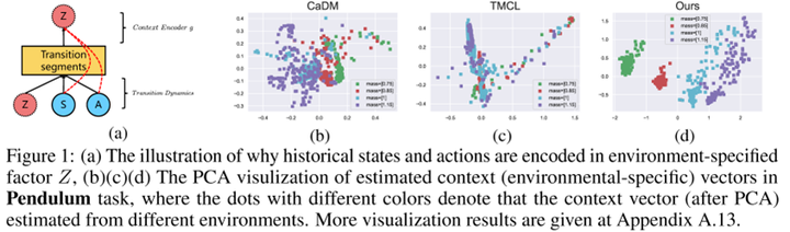
In this section, I will also explain some interesting ideas provided by causal RL using two works as examples. The first work is ‘A Relational Intervention Approach for Unsupervised Dynamics Generalization in Model-Based Reinforcement Learning,’⁸ presented at ICLR 2022. This work investigates the model generalization problem in MBRL, where context variables determining changes (such as weather, terrain, etc.) are unobservable. In traditional MBRL approaches, trajectory segments are commonly used to encode context information. However, this process tends to encode irrelevant information from states and actions into the context, thereby affecting the usefulness of the estimated context.

The author proposed a causality-inspired solution with the following framework:

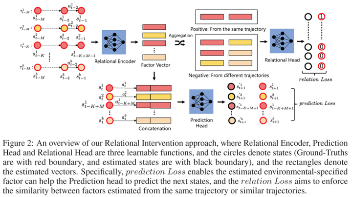
Firstly, the learning objective involves a prediction term, i.e., predicting the next state $S’$ based on the current state $S$, action $A$, and contextual information $Z$. Additionally, to understand how to encode context, there needs to be a relational term. Its aim is to make the contextual variables of steps within the same trajectory or from similar trajectories generated from the same environment as consistent as possible. The challenge here lies in determining whether trajectories come from the same environment. From a causal perspective, within the same environment, the causal effects of contextual variables on $S’$ should be similar. Therefore, we can use this causal effect to determine if steps belong to the same environment. Furthermore, there exist multiple causal paths from $Z$ to $S’$, such as $Z \rightarrow S \rightarrow S’$ and $Z \rightarrow A \rightarrow S’$. The authors suggest that these indirect paths are susceptible to noise. Therefore, they choose to measure the controlled direct effect (CDE), which is the causal effect transmitted solely through the direct path $Z \rightarrow S’$. Experiments indicate that this method not only reduces prediction errors in state transitions but also achieves excellent zero-shot generalization in new environments. Based on the PCA results in Figure 1, it’s evident that the learned contextual variables effectively capture environmental changes.

The second paper to be introduced was also presented at ICLR 2022, titled “AdaRL: What, Where, And How to Adapt in Transfer Reinforcement Learning.”⁹ This paper focuses on the problem of transfer learning in reinforcement learning. Specifically, during training, the agent can access multiple source domains, and during testing, it needs to achieve good performance with only a small number of samples from the target domain. The paper proposes a framework called AdaRL:

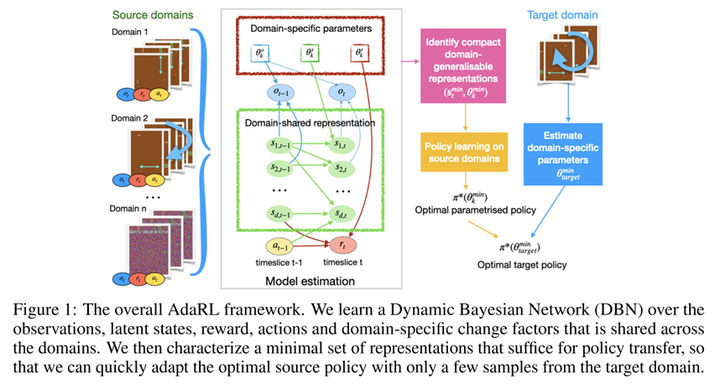
In particular, the author divides the model into domain-specific and domain-shared parts. The domain-specific parameters are low-dimensional, depicting variations of a specific domain. These variations can manifest in the model’s observations, states, and rewards within that specific domain. The domain-shared parameters include the causal relationships (edges on a causal graph) among different state dimensions, actions, and rewards, and their underlying causal mechanisms. By utilizing data from multiple source domains, agents can effectively learn causal models that can be reliably transferred as knowledge. Simultaneously, the low-dimensional domain-specific parameters require only a small number of samples from the target domain, making this framework highly flexible.

Spurious Correlations

Spurious correlation is a very common phenomenon, but traditional reinforcement learning rarely focuses on this issue. Below, we’ll use recommendation systems as an example to introduce two types of spurious correlations:

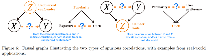
The first type is called confounding bias, where there might not be a causal relationship between two variables, but because of an unobservable confounding variable simultaneously affecting these two variables, they exhibit a strong correlation. The second type is termed selection bias, in which the association between two variables arises when considering a third variable. Techniques for analyzing and addressing these two types of issues in causal inference are well-established, so our primary concern lies in identifying the spurious correlations present in reinforcement learning problems.

Here, let’s delve deeper into the concept of confounding bias in policy learning through the paper ‘Causal Confusion in Imitation Learning’¹⁰ presented at NeurIPS 2019. Intuitively, we often believe that the more information available for decision-making, the better. For instance, using multimodal instead of unimodal data or constructing various feature interactions rather than using raw features. However, this paper introduces an intriguing idea: having more information isn’t always better:

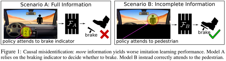
In this example depicted in the figure, the appearance of pedestrians is a confounding variable that causes both the brake light activation and the braking behavior. If an agent can observe the brake light, it might mistakenly believe that the brake light causes the act of braking. However, if the agent can only focus on the road ahead, it will correctly learn that the pedestrian in front is the actual cause of the braking behavior. If the agent learns the former, it will drive dangerously.

Meanwhile, our paper titled ‘False Correlation Reduction for Offline Reinforcement Learning,’¹¹ accepted by TPAMI this year, focuses on addressing spurious correlations in offline RL:

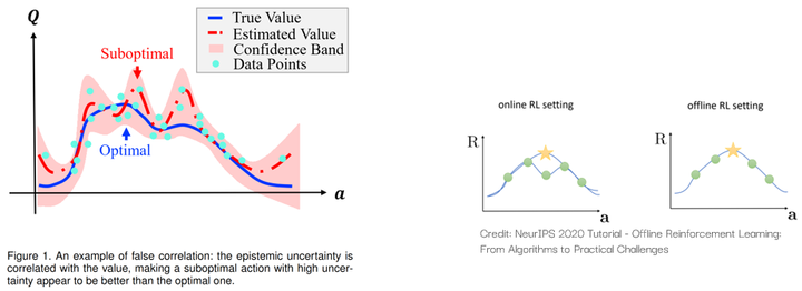
Due to the limited size of the sample set, the value of some suboptimal actions may appear ‘overrated.’ If an agent doesn’t consider the spurious correlations brought about by epistemic uncertainty, it may be influenced by these suboptimal actions, thereby failing to learn the optimal policy. For a detailed explanation, you can also refer to our blog posts for more details:

• 一篇顶刊论文背后的故事：TPAMI (2023) 用于离线强化学习的伪相关削减术 (Chinese version)
• The Insights and Story behind TPAMI (2023): False Correlation Reduction for Offline Reinforcement Learning

Explanaibility, Fairness, and Safety

Due to time constraints, I’ll update this section when I have more free time. Will try not to delay! 🕊️

Overall, we can summarize some common ideas provided by existing works in causal RL using the following diagram:

Limitations

So far, we have demonstrated the immense potential of causal RL methods in enhancing the decision-making capabilities of agents. However, it is not a panacea. Recognizing the limitations of existing methods is also important. One of the most significant limitations of Causal RL is its requirement for domain knowledge. Many causal RL methods rely on causal graphs, thus making accurate causal assumptions crucial. For instance, when dealing with confounding biases, some methods necessitate the use of proxy variables and instrumental variables, which, if not handled carefully, could potentially introduce additional risks.

Moreover, in some real-world scenarios, raw data is often highly unstructured, such as image and text data. The causal variables involved in the data generation process are usually unknown, necessitating the development of methods to extract meaningful causal representations from high-dimensional raw data – causal representation learning. These methods usually require learning from multi-domain data or allowing explicit interventions on environmental components to simulate the generation of intervention data. The quality and granularity of the learned representations heavily depend on available distributional shifts, interventions, or relevant signals, while real-world agents often only have access to a limited number of domains. Some methods not only aim to learn causal representations but also attempt to learn the underlying causal model, which is highly challenging. In some cases, learning a causal model might be more difficult than directly learning the optimal policy, potentially offsetting the gains in sample efficiency brought by using the model.

Finally, we need to acknowledge the limitations associated with counterfactual reasoning. Obtaining accurate and reliable counterfactual estimates often requires making strong assumptions about the underlying causal structure since, by definition, counterfactuals cannot be directly observed. Some counterfactual quantities are nearly impossible to identify, while others can be identified under appropriate assumptions, such as the effect of treatment on the treated (ETT). Additionally, the computational complexity of counterfactual reasoning is a bottleneck, especially when dealing with high-dimensional state and action spaces. This complexity might hinder real-time decision-making in complex tasks.

Resources

Prof. Elias Bareinboim¹² is one of the earliest scholars to systematically investigate the field of Causal RL. Many significant works in this field came from his research group. He initiated two tutorials at UAI 2019 and ICML 2020 respectively:

• 【Tutorial】Towards Causal Reinforcement Learning [Video] (UAI 2019)
• 【Tutorial】Towards Causal Reinforcement Learning [Video] (ICML 2020)

Dr. Chaochao Lu¹³ has also done excellent work in popularizing Causal RL. He believes that Causal RL is one of the pathways toward achieving Artificial General Intelligence (AGI):

• Causal Reinforcement Learning: A Road to Artificial General Intelligence [Slides]
• Causal Reinforcement Learning: Motivation, Concepts, Challenges, and Applications [Slides]

Prof. Yoshua Bengio has been actively promoting the development of the emerging field of causal representation learning in recent years. His collaborative paper with Prof. Bernhard Schölkopf¹⁴ also includes discussions related to Causal RL.

• Towards Causal Representation Learning [Slides]

Dr. Yan Zeng from Tsinghua University also wrote a survey on causal RL. Unlike the taxonomy taken in our survey, her paper categorizes existing work from the perspective of whether causal information is known, and we recommend reading the two papers together for a comprehensive understanding.

• A Survey on Causal Reinforcement Learning [Paper]

Finally, there was a tutorial we launched at ADMA 2023:

• 【Tutorial】Causal Reinforcement Learning: Empowering Agents with Causality [Slides]

For more resources, you can refer to our GitHub project. Feel free to give it a star ⭐️:

Awesome-Causal-RL: A curated list of causal reinforcement learning resources.

Afterword

Agents was a relatively niche concept when I began writing the survey, mainly discussed among scholars in the fields of reinforcement learning and robotics. However, in one year, accompanied by the wave triggered by ChatGPT, from the Stanford village¹⁵ released at the beginning of the year to the recent release of OpenAI’s GPTs store¹⁶, LLM-driven agents have demonstrated amazing levels of intelligence and tremendous commercial potential. This has not only sparked extensive discussions within academia but also garnered attention across various industries. Amidst this buzz, many researchers are exploring diverse research pathways and the relationship between agents and human beings. Besides multimodality and embodied intelligence, causality is also a great entry point. We anticipate that causal RL will showcase greater insights and play a larger role in the era of agents.

A quick advertisement: for those interested in Causal Reinforcement Learning, feel free to reach out! I’m also open to collaborating on new research papers and projects in this field!

Please check Zhihong Deng’s Homepage for further information. Thank you! Enjoy your day~ 😊

References